
The rock-scissors-paper game is simple, with one optimal mixed strategy for each player that consists of picking one of the three choices with equal frequency. The game is fair, favoring neither player. Nevertheless the game has a large following with many claims of how to win at the game.
Decision process theory has something to say here that sheds new light. The perspective is that the payoffs are not fixed for each player; there are negotiation forces that influence the choices to be made not only between players but for the same player. There are also valuation forces pushing the choices along individual strategy directions that need not be “classical game theory”.
Decision process theory predicts how these forces play out. Without going into the details of the computations, we gain insight into such such forces by analyzing the qualitative aspects of this simple game in the context of the theory. For this we use a simple “dashboard” below that allow us to change the payoffs and observe the equilibrium flow direction so implied. We hope that a full theoretical treatment would yield similar insights, while correcting any misperceptions that result from this rather simplified approach.
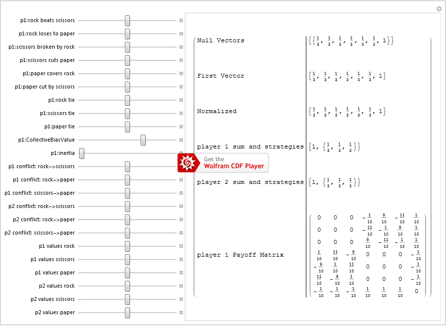
To experiment with this dashboard, download the Rock Scissors Paper cdf file after loading the free Wolfram CDF Reader. Note that the reader does not yet work on smart devices such as iPads.
Negotiation fields: in its simplest form, the game is played based on the idea that for each player, rock breaks (wins over) scissors, scissors cuts (wins over) paper and paper covers (wins over) rock. This is put into game theory format by saying that for each player, they see a unit payoff for each and the negative amount if they lose. If both players play the same thing, the payoff is zero. In game theory, the matrix is called the payoff matrix and appears as the 3-by-3 block matrix in the lower left of the dashboard, one up from the bottom row. The game can be made symmetric by creating the fiction that each person plays both sides: hence the payoff matrix (negative transpose) also appears at the top right, one to the left of the last row. The last row (and last column) represents a “hedge strategy” of the fictional game; it insures that the results of the fictional game exactly match the original payoff. In decision process theory, we take the fictional game as a non-fictional representation of the game with the “hedge” direction re-interpreted as time.
We retain the interpretation of the payoff, which we now call the negotiation field. We make this distinction because the field can change in time and can be thought of as a negotiation between the players. As in game theory, there is a distinct negotiation field matrix for each player, so that the time dependence reflects that player’s internal view of their own preferences and their opponent’s preferences. So for example if you (player p1) believe there is an increase in utility for “rock breaks scissors” from 1 to 2, your ideal strategies change from equal to {0.25, 0.333333, 0.416667} and your opponent (player p2) strategies change from equal to {0.333333, 0.25, 0.416667}. Your opponent should pick up on this preference and play paper more often. You on the other hand are forced to play rock less often because of the competitive nature of game: you play defensively.
Collective Bias Value: game theory makes no strategic distinction between games if their payoffs differ by an overall constant. We call this the collective bias value. You can verify that changing the collective bias value on the dashboard for the baseline case does not change the ideal strategies. The collective bias value for each player reflects a certain way of thinking about decision processes. In most cases, we make decisions assuming the utility of the decision is in our favor. We thus unconsciously add a collective bias value. So for example if you add a value of 0.1 to the payoffs, each payoff for you is positive and each payoff for your competitor is negative. On the dashboard, the collective bias value has been added as a convenient slide, saving you the trouble of moving each of the payoffs up by the same amount.
Valuation fields: In game theory, when defining the fictional game, when the collective bias has zero (game) value, the last row and the bottom column are zero. This last column (and last row) has values in general proportional to the game value. In decision process theory, we extend this concept. Because we label this column (and corresponding last row) time, the payoffs in this column we distinguish from the negotiation fields and call them the valuation fields. You can use the dashboard to see the ideal strategy in the case that the collective bias value is 0.1 and the valuation fields are 0.1 for player 2 and -0.1 for player 1. The players should have equal and opposite valuation fields because payoffs by their nature are competitive and implicitly zero sum.
We go further however. We see the valuation field for each strategy as generating a force along that strategy, since a player need not value each strategy the same. Set the collective bias value to 0.1, and all the valuations to 0.1. Now change “p2 values rock” from 0.1 to 0.2. This makes no change to your opponent’s (p2) ideal strategies, but does change your (p1) strategies from equal to {0.333333, 0.308333, 0.358333}. This says that you have learned of your opponent’s leaning towards picking rock. It is a bias on your opponent’s part. If you pick paper you will clearly gain an advantage based on your knowledge of your opponent’s bias.
On the other hand, let us say that you (p1) decide to place more valuation on rock and your opponent does not. You change your “p1 values rock” from 0.1 to 0.2. Your ideal strategy does not change this time but your opponent’s does: {0.333333, 0.358333, 0.308333}. It is not symmetric however. The reason is that your valuation of rock moves you towards the origin, toward preferring rock less. This will be compensated by your negotiation forces. This means your opponent can take advantage of your bias by picking paper less, since there is less concern you will pick that. This is compensated by choosing scissors more. Note that in these last two examples, the total rate of making choices is larger for the other player, the player that does not increase their choice.
Inertia: a related attribute of valuation fields and the collective bias value can be seen on the dashboard choice of the “normalized” ideal strategy. The normalization is to pick the time component to be unity. This allows us to make comparisons for different models. Since we argue that increasing the collective bias value should increase the valuation fields, by holding the fields constant we implicitly introduce a new parameter we call the inertia: the ratio of the collective bias value and inertia are thus being held constant. A consequence of this is that the normalized ideal strategy will have “flows” that get smaller as we raise the collective bias value. This substantiates our view that the strategies are the rate of change of preferences in response to the valuation and negotiation forces. A high inertia corresponds to very slow movement.
Internal negotiation fields: A distinct difference between our approach here and game theory is the possibility of capturing internal conflicts, factions and self-payoffs. Suppose our opponent (p2) decides that she is in cyclic conflict over rock and paper in a way which is totally internal. On the dashboard move the slider for this possibility from 0 to 0.2. She has no reason to suppose in this case that we have made any changes in our utilities, so her ideal strategy stays the same. However we may profit from this internal cyclic conflict as seen by our ideal strategy: {0.355556, 0.288889, 0.355556}. We decrease our frequency for scissors to capitalize on the area of conflict.
Ideal strategies and forces: Our approach here has been to identify mechanisms that generate change. We call these forces. So for example, the negotiation field component {i,j} generates a force on our (p1) choices along the “i” direction as a negotiation between our choice and our opponent’s choice along the “j” direction. This is rather different from the valuation force for the component “i” that generates a force along the same direction independent of what our opponent does. When these two types of forces exactly cancel for every strategy, there are no forces moving either our strategies or our opponent’s strategies in either direction, defining an equilibrium position we call the ideal strategy.