Introduction
This talk was given at the Wolfram Technology Conference in October 2014 at Champagne, Illinois. The idea of the talk was to explore how one visualizes behaviors in differential geometries that are more complex than the usual three-dimensional flat geometries we are familiar with.
Abstract
We use Mathematica to visualize such behaviors. Our access to these behaviors are the partial differential equations that describe the shape of the geometry; these equations provide us a way to track the shortest paths. Shortest path algorithms are familiar from Newtonian mechanics, geometrical optics, Maxwell’s theory of electromagnetism and Einstein’s theory of relativity. My particular interest has been the possibility of using the shortest path algorithms of differential geometry to solve problems in the social sciences; in particular to gain insight into the causal behavior of decision processes. In this case, the starting point is the conjecture that decisions are events that form a continuous manifold in both time (causality) and space (strategies). This is a fundamentally different starting point from the usual stochastic approaches used in the social sciences. The resultant behaviors are shortest paths in a differential geometry space.
The challenge is to visualize these behaviors that are consequences of the differential geometry. This talk addresses that challenge. We apply Mathematica solutions to the partial differential equations and look at limit cycles and limit surfaces and their relationship to harmonic solutions and chaotic behaviors. We proceed with model solutions using Mathematica of more complicated differential geometry possibilities that have applications to gravitational theories and decision theories. We find that the NDSolve and Manipulate functionality can be used to great advantage in order to visualize the behaviors in these geometries. There are many other applications of these visualizations, such as teaching possibilities in Electro-Magnetism courses.
Outline of talk
- Decisions as Geometry
- Take an example www (work-wealth-wisdom) model
- What is time? What are space components? How is uncertainty dealt with?
- Idiosyncratic behavior and symmetry
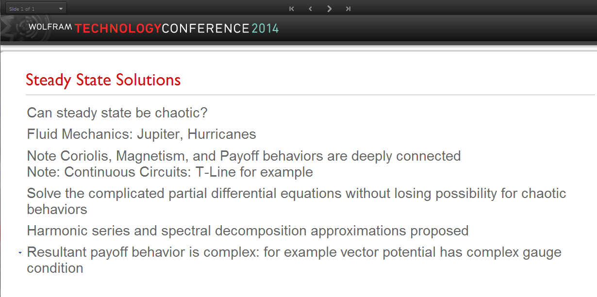
- Steady state solutions
- Can steady state be chaotic? Jupiter red spot!
- Examples from WWW–rotations, Coriolis, magnetic fields and payoffs
- Need to solve complex stationary problem
- Use harmonic series approximation
- Do we exclude chaotic behaviors? See toy model . Build on this with harmonic solutions
- Decision geometry is more complicated than in physics
- Two different transformations to stationary frame–two versions of time flow
- Communication travels at a finite speed
- There are communication ellipses
Decisions as Geometry
There are many examples of geometry in the physical world, starting with the most familiar, the geometry of the earth. Many theories, such as Newtonian mechanics use geometry in a variety of contexts that extend the notion of purely flat space to spaces with curvature. The most striking example is perhaps the theory of Einstein, which maintains that our “normal” space is 3+1 curved dimensions. The specific behaviors of geometry that we find interesting are:
- Position and Uncertainty
- The nature of time
- Symmetries
These are particularly interesting to us because of the possibility of using geometry to describe how we make ordinary decisions in the business and economic world. We have presented these ideas at past Wolfram Technology Conferences; many more details can be found on my website.
Position and uncertainty: Let’s deal with position and uncertainty first. At least some of us think of position as described in physical laws as certain, and think of “soft” concepts such as decisions as inherently uncertain. That is perhaps not the full story. It is true that at least starting with Newtonian physics, the concept of position is considered as something that is well-defined and certain. However, the measurement of position is not. Anyone that has measured a room knows that every time you make the measurement you get a slightly different number. Thus the key insight in Newtonian mechanics is to separate the concept of position from measurement: the certain concept from the concept that has a degree of intrinsic uncertainty.
We suggest a similar type of split is necessary for considering decision making, a split that has been made in the Theory of Games. The concept of utility can be applied to preferences as a well-defined concept of certainty. However the measurement of preferences involves observing the frequency with which we make our choices. For any given decision point, we make one choice out of several, which is uncertain. Nevertheless our preferences, like position, might be considered as certain. As with game theory, we take as a point in space, the collective strategic preferences of each decision maker.
Time: Let’s deal with time next. In physical processes, we can think of time as Newtonian, meaning we ascribe an absolute time as being applicable to all events happening anywhere throughout the universe. Alternatively, we can think of time as Mawellian, meaning we ascribe a local time to the events happening in our vicinity, and potentially a different time for events happening elsewhere. It seems to be a less efficient way of talking about time, but does allow for the fundamental fact in Maxwell’s description of light that light travels at the same speed regardless of frame of reference. Einstein took up this argument and concluded that in this respect Newtonian mechanics needed to be modified to conform with Maxwell’s description.
As a rule, we describe physical processes as causal in nature. Once we agree on a definition of time, we incorporate that description into the way we see the world. Events happen in succession with earlier events having the possibility of influencing later events in a strict cause and effect relationship. Not all events have such a relationship. Statistical events may occur in such a way that later events are independent of all earlier events. A particular type of such an event is stochastic. Wikipedia says: “In probability theory, a purely stochastic system is one whose state is non-deterministic (i.e., “random”) so that the subsequent state of the system is determined probabilistically. Any system or process that must be analyzed using probability theory is stochastic at least in part.[1][2] Stochastic systems and processes play a fundamental role in mathematical models of phenomena in many fields of science, engineering, and economics.”
What stance do we take? Do we assume a causal behavior or a stochastic behavior? The current literature favors the idea that decisions reflect stochastic processes. We take the opposite point of view: We follow the lead from those that have applied Systems Dynamics to a variety of real world problems and conclude that many real world problems can be treated as causal. Having taken this stance, the next question is whether we take a Newtonian view or a Maxwellian view. We have studied decisions starting from the formulations of the Theory of Games and note that the underlying concept of payoffs closely parallels the concept of magnetic fields and so adopt the Maxwellian point of view.
The key conclusions we make for our study of geometry of decisions is that it be based on positions as determined by strategic preferences and time as a local variable subject to the constraint that information move at a speed that is locally the same to every observer in the system. This is similar to the geometries envisioned by Einstein in his theory of general relativity. It is much broader however in that the number of dimensions is not limited, but depends on the number of pure strategies available to the collective of decision makers. The local nature of space and time so defined relies on the existence at each point of a set of potential fields, one for each dimension of space and time. A surface of constant potential is one on which we have a single well-defined value for the amount of distance or time is appropriate to that coordinate. We can call these coordinate surfaces. On a map of the earth, these would be the lines of constant latitude or constant longitude; these have a meaning on a flat chart despite the fact that the lines represent a spherical (or oblate spherical) earth. In higher dimensions these lines we call hyper-surfaces, or simply surfaces.
Symmetry and idiosyncratic behavior: Common physical systems often exhibit symmetries that are an essential part of how we think of them. The earth is symmetric about its axis; indeed it is almost spherically symmetric. Such symmetries are reflected in the way we describe the geometry. Let’s pursue as an example the axial symmetry of the earth. The oblate character is reflected in the behavior of the latitudes and the symmetry is reflected in the way we treat the longitude. There is no difference in the shape of the earth at different longitudes. Newtonian physics provides deeper insights: there is a theorem from physics and geometry that to each symmetry there is a conserved motion, which in this case is the angular momentum. It can be shown that the law of sines in trigonometry is a consequence of this conservation law. It is a further attribute of differential geometries that there will also be two associated forces: a centripetal scalar force and a Coriolis vector force. Identifying symmetries provides substantial insight into the geometry. In many cases, the symmetries are not immediately evident, though the attributes are. Locally, we may notice the Coriolis forces before we notice that the earth is not flat.
We also believe that there are important “symmetries” in decision-making, though as with the curvature of the earth, it may be that the attributes or consequences of the symmetries are more noticeable than the symmetries themselves. We find it notable that the game theory approach to decision-making uses the Nash equilibrium, a static scenario in which each player considers his or her version of the game, considers all the worst consequences that can happen, and from those chooses the best of the worst. It is often framed as a max-min choice. It is an equilibrium in the sense that every player makes the same type of choice, and no other choice works better for any player.
The idea we take away from this is that first, it is idiosyncratic: it is based on each player’s personal view of the utilities. Second, the max-min choice has relevant mathematical connections to geometry: the dynamic path or motion in a rotating frame has one “equilibrium” direction parallel to the rotation axis, which can be framed as a max-min solution to motion. Motion in any other direction will be influenced by apparent or Coriolis forces. For this talk, we don’t go into detail other than quoting the result that if we associate with each player a symmetry, then the consequence will be that there will be a game matrix associated with that player that dictates the relative utilities and there will be an equilibrium set by a max-min choice.
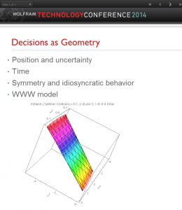
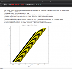
WWW model: with these preliminaries of geometry out of the way we can briefly describe the decision model we will use as an example of complicated geometries. We call it the Work-Wealth-Wisdom model. The various figures or CDF models, such as the one above, have been computed based on the explicit model and numerical values chosen.
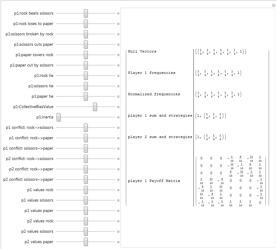
One common way in game theory to formulate a decision is to specify a matrix that indicates the payoffs. The rows correspond to the choices of one player and the columns the other player. From a mathematical perspective, this can be reformulated as a symmetric game in which the rows specify the choice of every player plus one additional row called the hedge strategy, and the columns also specify the choice of every player and one additional column called the hedge strategy.

This is the symmetric version of the payoff strategy for the WWW model. The model shown here is totally illustrative and the numerical values could be chosen quite differently. There are two players: the work-player and the wealth-player. Wisdom is how they play the game. The order of the rows (columns) reflect the wealth-player (player 2) strategy to invest wealth into the economy or to collect rent, then the work-player (player 1) strategy to earn or to “take” money, then finally the “hedge” strategy that we identify with time.
The model incorporates the idea that wealth has 10 times more value than the work and the consequence is that there are 10 times more workers than wealthy. The payoff to the worker is 1 if their choice is “work” and the wealth choice is “invest”. The worker gets nothing if the wealth choice is to collect rent. The payoff to the worker is 0 if the worker chooses to “take” and the wealth choice is “invest”. The payoff is 1/10 if the wealth choice is to “rent”. In the sense of game theory, no pure choice forms an equilibrium. The best choice for the work-player is to pick either choice with a 10:1 choice favoring “take”. The best choice for the wealth-player is a 10:1 choice favoring “collect rent”. From the standpoint of game theory, this is where we stop, except that we have a second game matrix for the wealth-player that is in principle independent. That is the sense that the choices are idiosyncratic.
In a decision geometry, the symmetric payoff matrix is in fact a rotation in the space of strategic decisions consisting of the two choices for the work-player, two choices for the wealth-player, two hidden dimensions reflecting the symmetry which generates each of the two payoff matrices and time. The space is seven dimensional, in which only five of the dimensions are “active” or not hidden. In our model, we assume that the sum over all the active strategies is a symmetry, leaving us with a four dimensional world in which three are “space” and one dimension is “time”. The model is thus parallel in some respects to the physical world we live in. This is purely for numerical convenience and helps us visualize what is going on more easily.
Geometry: It is worth noting that the concept of payoffs arises entirely from an inquiry into utility and economic behaviors. However from a mathematical point of view, we see it as a hint of an underlying geometry. It is possible to use mathematics to relate the payoffs to a concept of distance between points in this strategic space-time. We thus move the ideas above from a concept of coordinate strategic surfaces to the concept of a function of such coordinates that define a distance function on the space-time manifold. The payoffs are then just one aspect of this distance function. This is the context in which we view decisions as geometry.
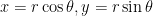
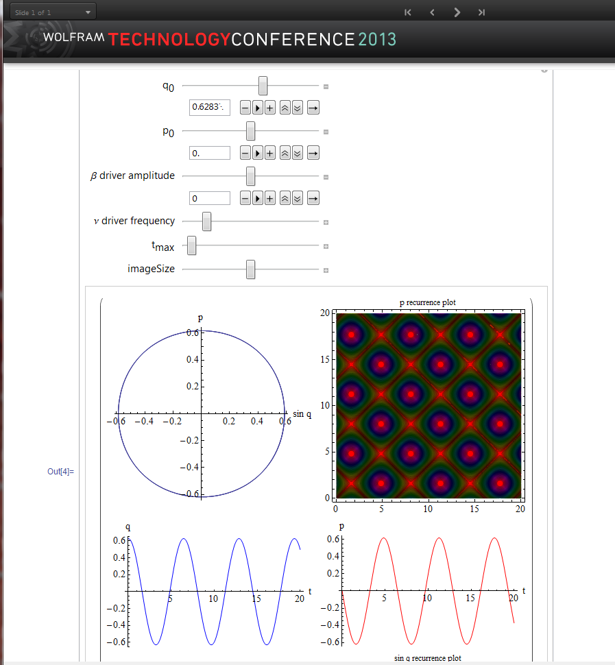
Visualization: The resultant geometry is one whose structure changes over time in a well-defined way. Our challenge is to describe that change in a way that makes sense and can be pictured. An example may help: the surface of the ocean is an example of something whose shape changes as a function of time. On the one hand, in the normal coordinates of viewing, we see the shape constantly changing. On the other hand, there are behaviors that can be more simply described if we imagine we are a cork riding on the surface: from our co-moving perspective everything is stationary, though we see structures that when related to the normal coordinates appear as dynamic structures such as waves. We find the same is true in our general geometry. There are many types of solutions, some of which allow a co-moving description that is stationary. Though stationary or steady-state, the motion described is still dynamically interesting: we get standing waves for example. The steady-state motion is what happens after all transient effects die out. For the WWW model, we have positions in the co-moving frame that we call x, y and z as well as a proper time  . These relate back to normal coordinates of
  . This will be our first type of visualization.
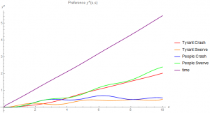
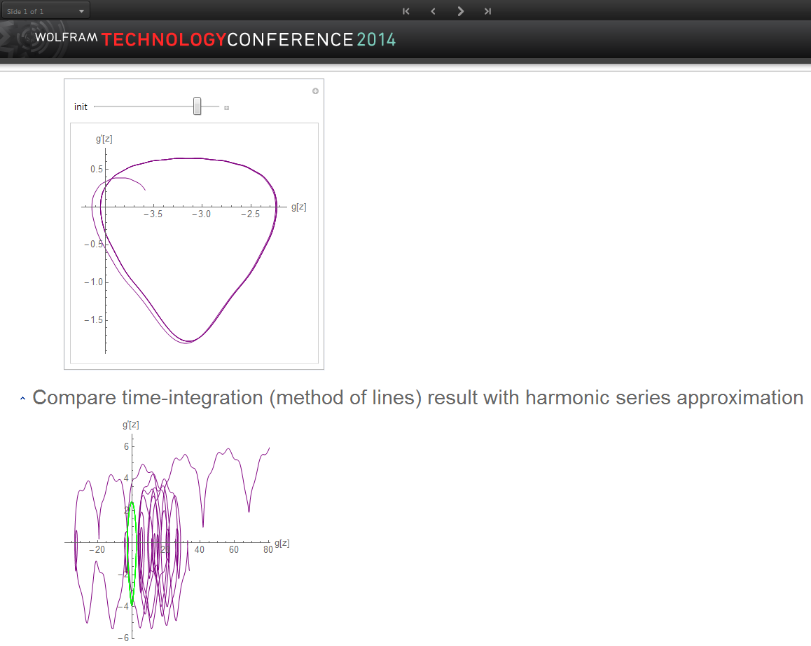
So for example with x and y constrained to be on a circle with fixed radius and arbitrary angle (a cylinder), we can ask what that behavior looks like in normal coordinates. That is shown above. We can also look at the velocity flow,  against t, as contours as shown below. For the WWW model, the income inequality generates a corresponding velocity. What are the normal coordinates here? The direction
  is the relative preference for “work” versus “take”; the direction
  is the relative preference for “invest” versus “rent collection”; the direction is the relative intensity with which each player plays the game, work minus wealth. So in the graph below, the vertical axis is time and the horizontal axis is . The strong direction along the horizontal axis reflects the increase in workers needed because of the assignment of value to wealth. This was put in as an initial condition; the model then shows the consequence of this assumption over time. Note that co-moving time contours are not constant in normal time. This reflects our way of dealing with time as similar to that of Maxwellian and not Newtonian theories.
Steady-State Solutions
One way to characterize a geometry is by how one measures distances. For example we may use flat maps to plot a course over the ocean. On this map, the latitude and longitude may appear as orthogonal straight lines. However for an accurate course, we need to know how to relate these lines to distance; if we go far enough the distance is not Euclidean since the earth is approximately an oblate spheroid. Another way to characterize a geometry is to plot the paths that represent the shortest distance between two points. It is derived from the distance measure and reflects the curvature of the space. Thus, we may study the complexity of the geometry either by the shape of the surface or by the shortest paths. A complicated geometry is one in which the paths are complex. An example from weather might suggest what we have in mind: a hurricane or tornado both have cyclonic paths of wind, suggesting chaotic behavior. Ordinarily we associate chaotic behavior to the time dependence of the flow. Yet we can have cyclonic behavior that appears stationary. A good example of such a flow is the “spot” on Jupiter that has been around for centuries. In this talk we focus on such steady-state behaviors that remain after any transient effects die out. Of course there will also be behaviors associated with the transients, but they are the subject of a future investigation.

We suggest that the origin of complex behaviors, such as chaotic behaviors, are similar in different domains of study, be they weather phenomena, electromagnetic phenomena or decision phenomena. In each case there are symmetries that give rise to Coriolis forces, magnetic forces or payoff forces respectively. These forces arise from common differential geometry structures.
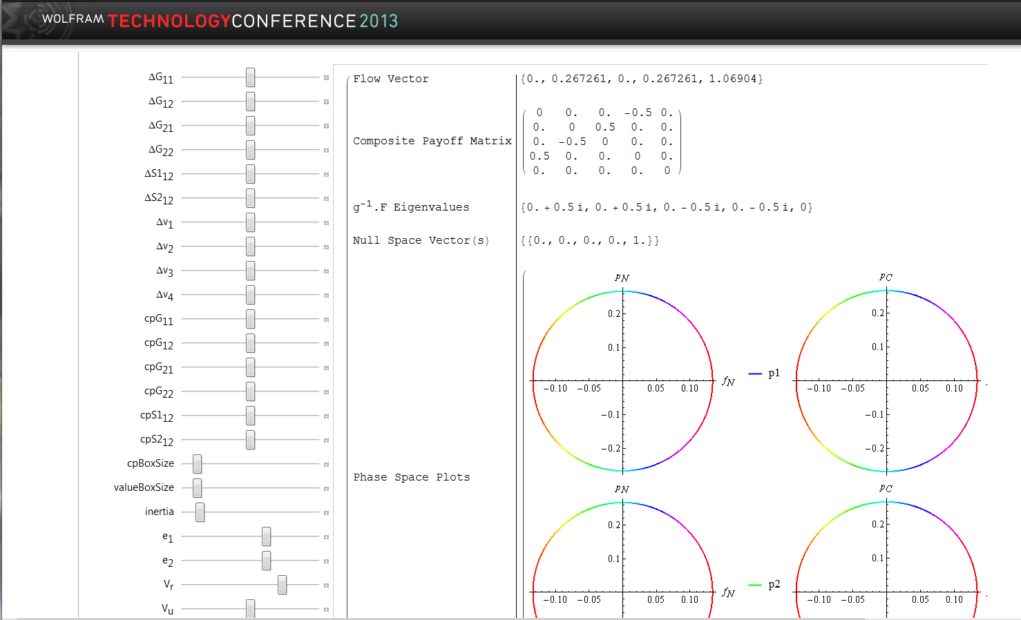
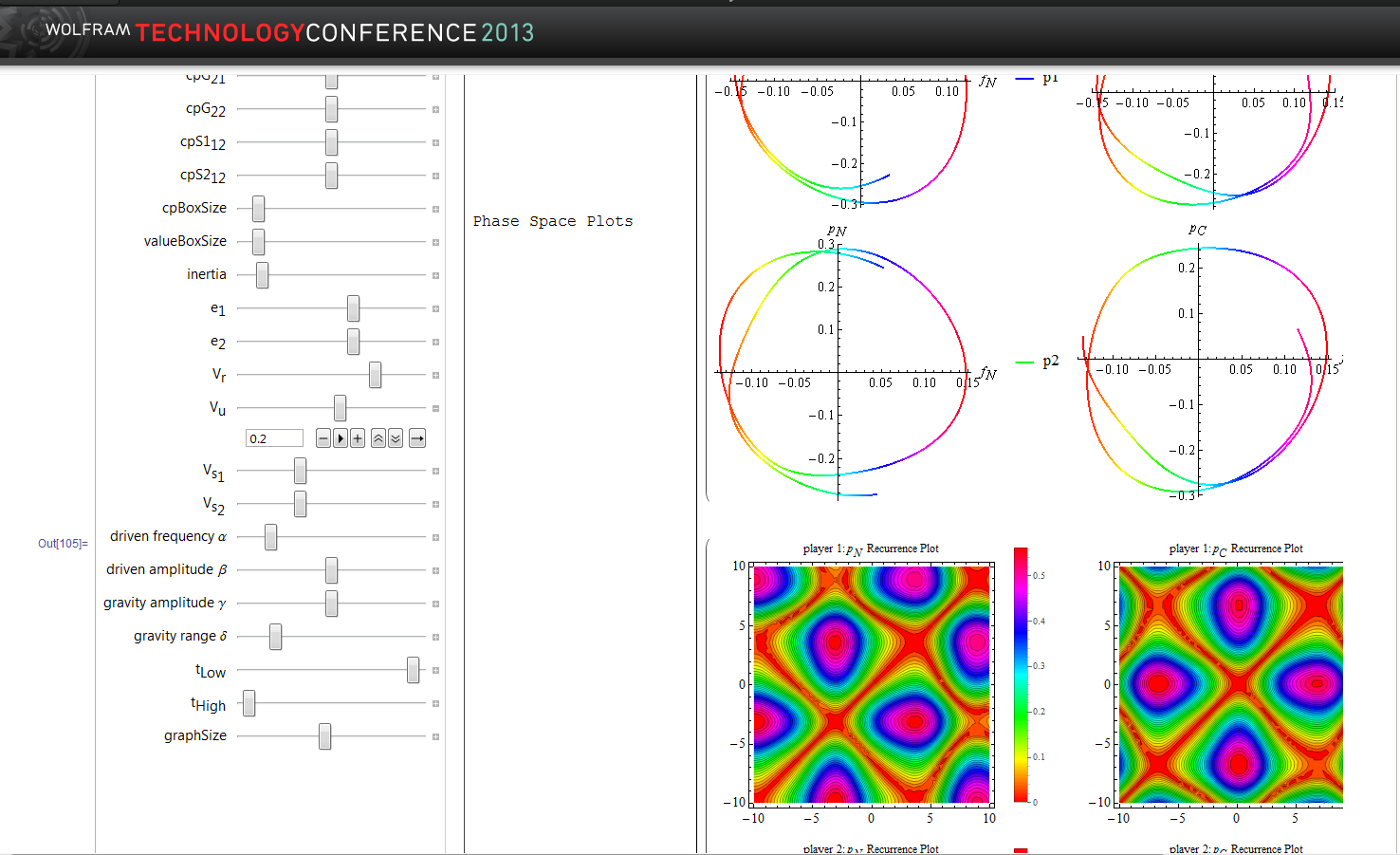
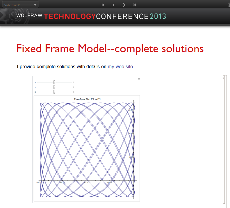
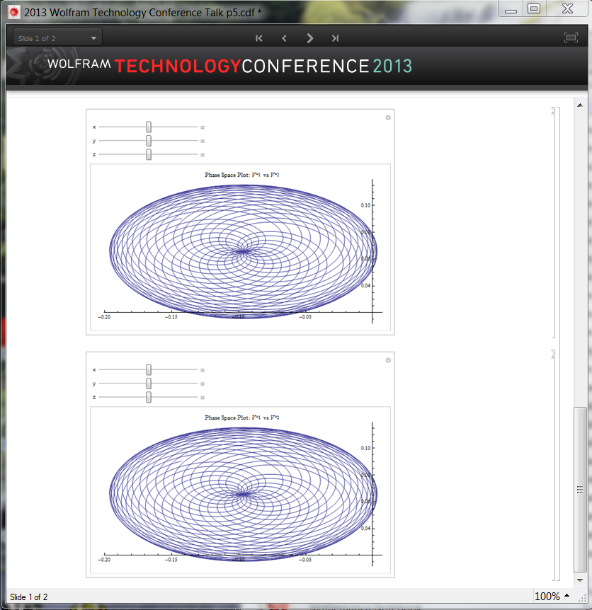
To study these structures we would start with the fact that the cyclonic behaviors are the result of rotations and such rotations can be investigated by looking at the fields that generate the rotations. The following shows a “phase space” plot of the fields from the WWW model that are used to generate the overall payoff matrix.
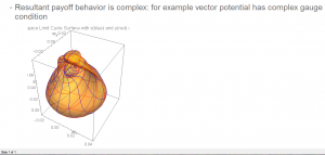
This field is anything but simple. The CDF picture can be rotated showing the type of complexity one might get. For the experts, we note that this picture is the set of limit surfaces for the z component of the gauge field, along with the partial derivatives of that gauge field along the other two transverse directions x and y. A sphere would be the 3-dimensional analog of a circular phase space plot in 2-dimensions , which is quite different from what is shown here.
Steady-State Solutions can be chaotic
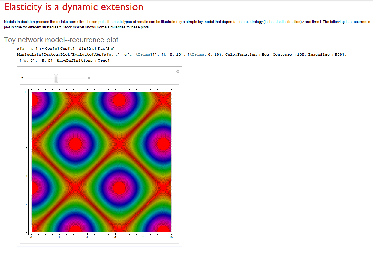
Of course the solutions that we obtain for a geometry may depend on the assumptions used to do the numerical work. So we take a step back and analyze the types of assumptions that we have made. Our tentative conclusion is that we can apply a “harmonic-series” approximation and still identify chaotic solutions. This follows from a technical discussion using Mathematica as a computational tool.
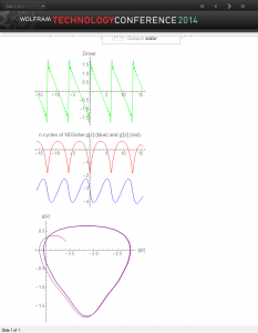
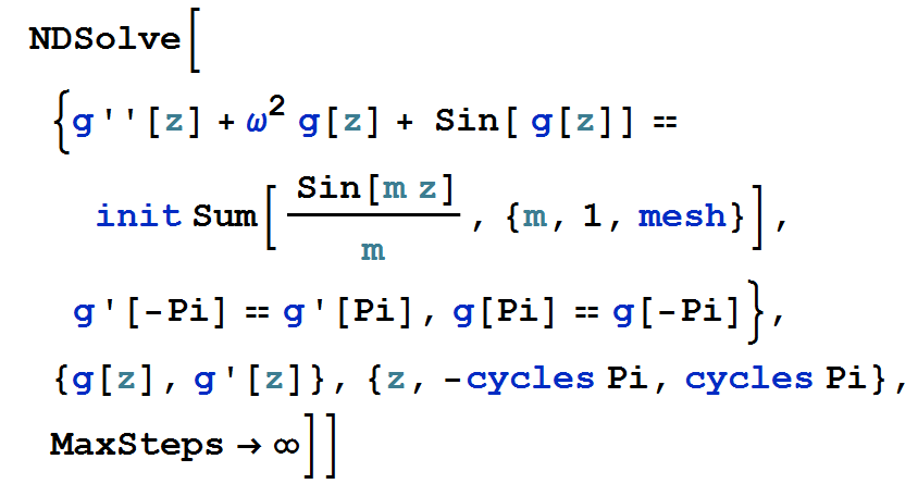
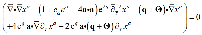
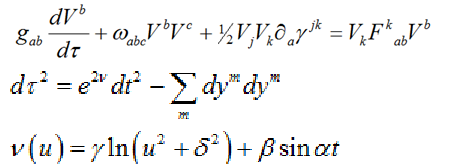
Consider a gravitational source equation with non-linear terms:

The source, which is the first figure above (green curve) is periodic and for illustration is a saw-tooth pattern. We scale it by a factor, init, which we vary. The equation is solved using NDSolve from Mathematica using periodic boundary conditions. It uses the method of lines to compute the function, red curve, and its derivative, the blue curve. For a sufficiently small factor value of init, the phase space plot shown in purple is a closed cycle. However past a critical value, the non-linear nature of the equation asserts itself and we cease to have closed cycle. We suggest this is the start of chaotic behavior, though we haven’t used a rigorous definition to establish this suggestion yet. The factor value chosen in this figure is init=1.7.

Use Manipulate to make chaotic behavior visible
The Manipulate function in Mathematica is a way to explore when the phase space plot ceases to be a limit cycle. We have considered different source terms, and in particular explored approximating the saw-tooth behavior as a Fourier series with a finite number of terms.
We need not extend the harmonic approximation to the solution. As noted above we use the methods of lines to obtain our full result. For more general geometries, we have also use periodic boundary conditions for all but one space direction. For time, we have considered a single Fourier frequency. For the remaining space direction we use NDSolve and the methods of lines.
General geometries however, may impose differential constraints on initial conditions. On the initial boundary we may have to solve a differential equation in one or more dimensions. The boundary conditions we may need to impose may also be periodic. Now however, the method of lines may not work if there are two or more independent coordinates. So what do we do?
Our solution was to expand the unknown functions as a harmonic series with unknown coefficients. We then substitute the function and its derivatives into the differential equations and use FindRoot to obtain the numerical values of the coefficients. In one dimension we can also use the method of lines as a comparison.
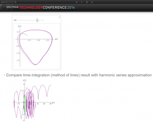
So, returning to the simple gravity source equation above, with a clearly chaotic behavior, purple curve, we also solve the same system using the harmonic approximation, green curve. Not surprisingly, the harmonic approximation is always a limit cycle. We see that the cycle fits into the more general solution. By changing the start point for FindRoot, we have found other limit cycles. So the chaotic behavior manifests itself in the harmonic approximation as multiple solutions.
For the decision geometry WWW model, using the harmonic series approximation, we get the limit surface, that we described earlier:
That it is a surface and not a hyper-curve is a consequence of it being a harmonic series approximation. However, the specific surface may depend on the “sources”.
Steady-state analysis: We can now describe more fully the steady state analysis that we perform for differential geometries. We illustrate the technique using an example in one time and one space dimension:

This form of a “wave equation” is typical of the harmonic gauge choice that is always possible to make in a differential geometry. The concept of steady-state is similar to that in electrical and mechanical engineering: As long as the functions A and B are functions only of the space variable z, we can replace the coordinate function with the product of a harmonic in time and an unknown function of space:

In other words, the harmonic gauge is then a linear equation in the coordinate. This reduces the partial differential equations to one of lower degree, one that is elliptic and depends on the frequency chosen. It has the form:

When there is more than one spatial dimension, the coefficients A and B depend on the coordinate so these become coupled elliptic partial differential equations. An example is the three spatial dimension model with one time:
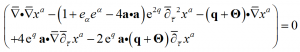
This steady-state solution could be viewed as a solution to a model from general relativity, decision process theory, or in fact any differential geometry model with three space and one time dimension. The boundary and initial conditions, however, will be specific to the problem domain.
We solve these equations using NDSolve, periodic boundary conditions for all but one spatial direction, and use the method of lines for the remaining direction. Constraint differential equations for the coefficients on the initial surface (all spatial directions but that reserved for the method of lines) will be solved using the harmonic series approximation to ensure that the coefficients remain periodic on the boundary.
Based on our investigations to date, we expect that the resultant solutions have the possibility of exhibiting not only “linear” and “near linear” solutions corresponding to simple limit surfaces, but more complex behaviors corresponding to chaotic-type behaviors such as space filling curves. We hope to be able to investigate what we believe is a quite rich structure embedded in these differential geometries. Our remaining examples will be taken from decision process theory, and in particular from the WWW decision model. We will focus on only two aspects out of what is in fact a vast wealth of possibilities: time and communication.
Decision geometry is more complicated than Newtonian physics
We start with a consideration of time and what it means in a differential geometry that consists of a generalized notion of time and space. We have a number of questions:
- Which way does time flow? Yes we know it increases and we know it moves in some sense orthogonal to space, but in which direction is that?
- Do we define the direction of time flow along the normal to the surface of constant time?
- Do we define the direction of time as being orthogonal to a spatial volume element? The volume,
 , is the wedge product generalization to the “cross product”
- Are these two directions the same or different in a general geometry
- Which way are they in the WWW model?
- How does the velocity we call
 help us understand and visualize the distinctions?
Time direction: In Newtonian physics, the physics that perhaps comes closest to the way most of us were raised, time clearly moves forward and never backward. Moreover, it is clear that time is orthogonal to all of the directions of space: up and down; forward and backward; left and right. Starting from this perspective, we construct our geometry, which is Euclidean in nature. Time flows and has a value that is the same everywhere in space. We have no real evidence of course that this is true. In fact, modern physics experiments demonstrate that this is not true. It is not that our ideas are unfounded, but that we have attempted to extrapolate our ideas too far beyond what we have observed.
We observe time locally, just as we measure distances in space locally. In our current location, what we mean by a coordinate is a value that is the same in a small region around where we are, at the current time. What we mean by time is a small region around where we are where a common clock suffices to provide a value for the current time. Putting these ideas into mathematics is brings us to differential geometry. In this discipline, we talk about a surface on which a coordinate is constant. Such surfaces exist at each point and extend to a region around that point. The region is not arbitrarily large however; it depends on the curvature and topology of the space. For a Euclidean space-time, the region does in fact extend everywhere. For curved space this is not the case.
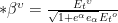
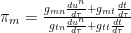
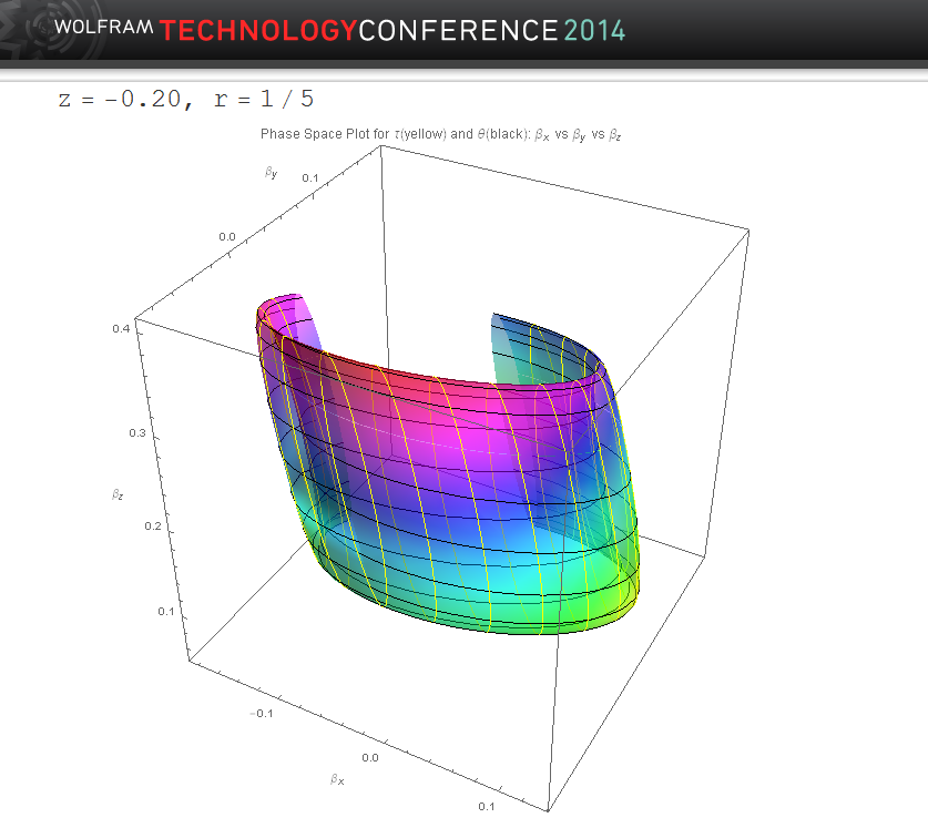
Normal time: From this mathematical perspective, we might then define the direction of time at each point as being along the normal to the coordinate surface associated with time at that point. For the steady-state WWW model, we can say more. The flow in that model is stationary in the co-moving frame. So at each point, we can say that the normal of the time surface is along that flow; the flow is moving at a certain velocity, which can be normalized as the ratio of the co-moving space component of flow divided by the co-moving time component of flow:

This is the . The additional square root in the denominator accounts for the energy due to the inactive component of flows that are associated with the idiosyncratic symmetries. The subscript in the numerator reflects the co-moving space components; the subscript in the denominator reflects the co-moving time component of flow.
We denote the co-moving directions as x, y and z; z is the direction in which we use the method of lines and the other two directions are transverse in which we use periodic boundary conditions. It is thus very natural to consider not x and y, but the radial directions such that
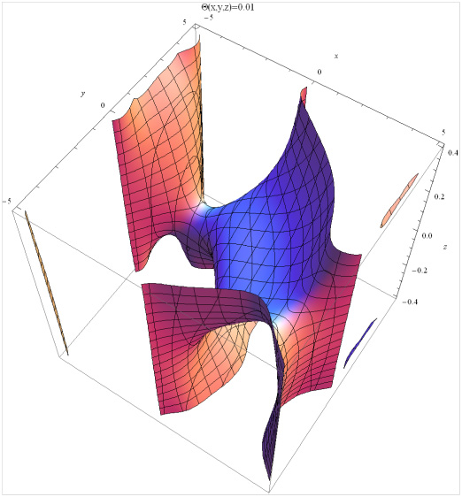
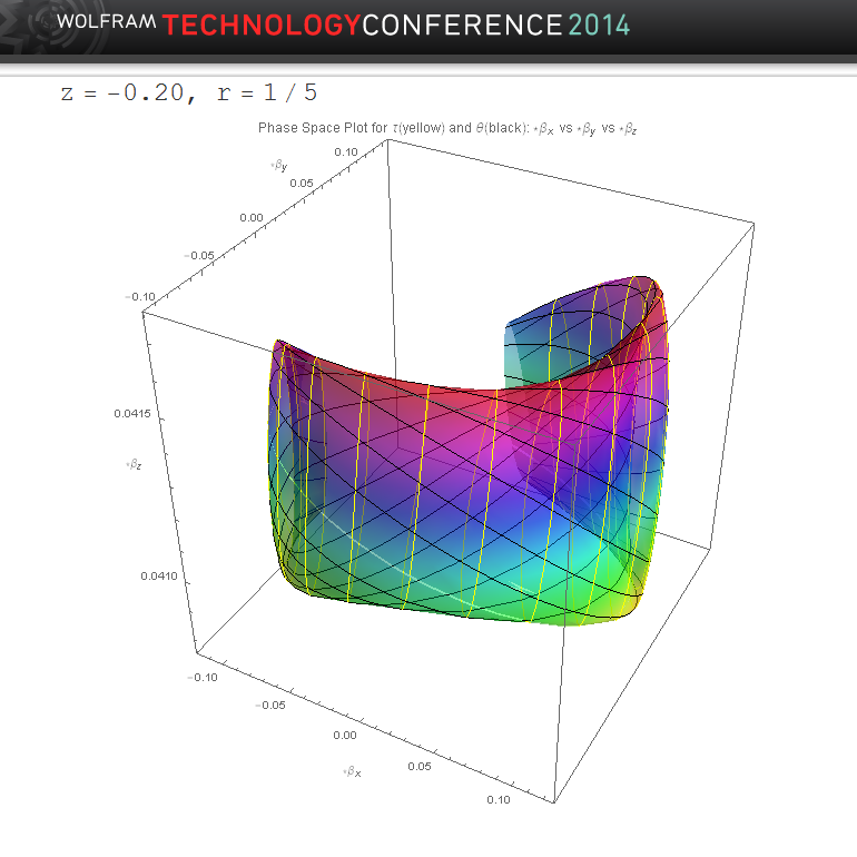
Using this notation, we can fix the radius to a number and look at solutions for all angles. We thus map a cylinder in the co-moving space into a two-dimensional surface in the “velocity” space associated with one concept of time.
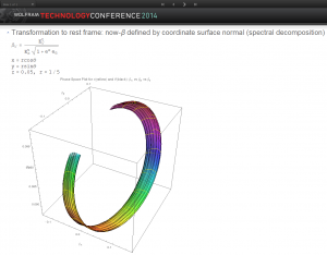
The image above shows this surface for r=0.2 and z=0.05; the CDF file provides an interactive way to view the same surface.

This figure shows the “velocity” surface at a different point, r=0.2 and z=-0.20. The two surfaces are quite different. If the flow were the same at every point, we would conclude that the geometry and time flow reflect some simple property such as the system is moving uniformly without rotation. This is clearly not the case.
Orthogonal time: Now let’s pursue a different approach, which is to consider that time flows in a direction normal to the space. To give this meaning, note that we are used to considering a small volume of space at each point and associating physical facts to such volume; the volume itself, the mass contained on that volume, the total utility associated with that volume, etc. Differential geometry also considers volumes, starting from the notion of a surface spanned by two coordinates, say x and y. The normal to the surface for x is a differential change dx; similarly the normal to the surface for y is dy. The surface area however spanned by dx and dy is related to the product, called the wedge product between the two:  . It is the anti-symmetric product of the two vectors. The volume is the wedge product of any three independent normals: . It is the anti-symmetric product of all three.
In differential geometry, we form the dual to any wedge product by a rule that constructs a totally anti-symmetric product of the given wedge product and adjoining all the remaining directions in an anti-symmetric way. In a four dimensional space-time, the dual of the volume is a one dimensional vector:

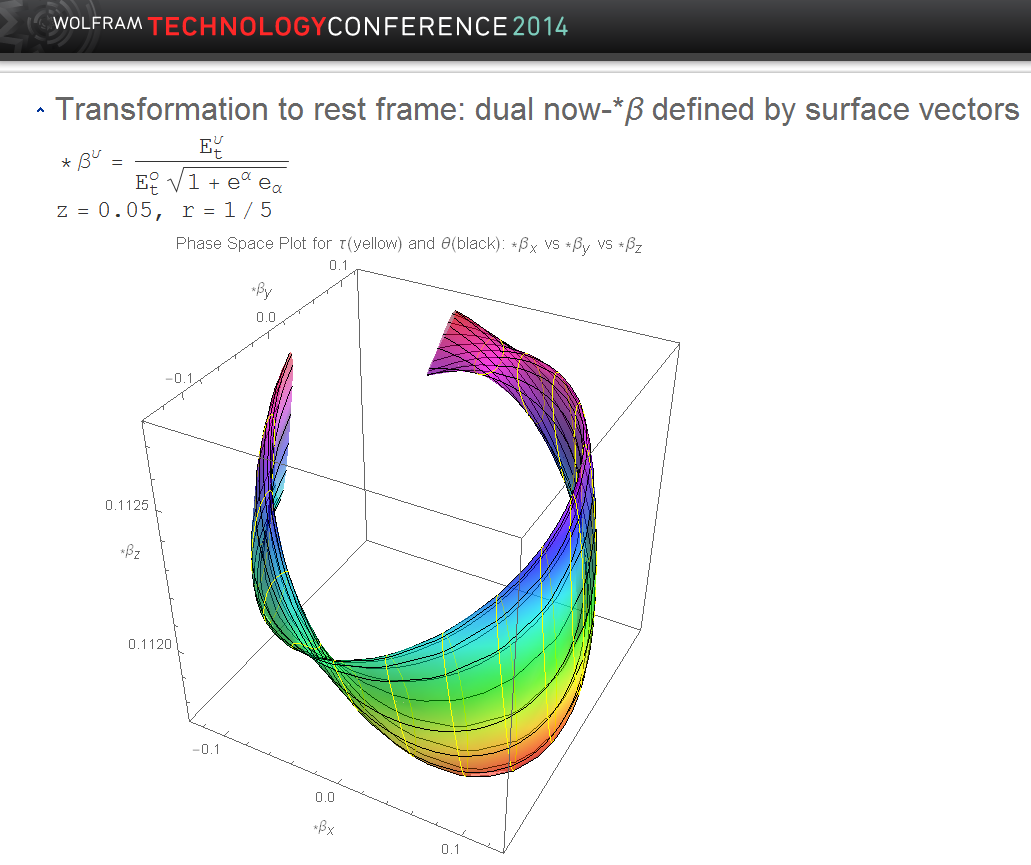
In general, hyper-volumes are described by forms. They generalize the cross product to higher dimensions. In particular, the direction orthogonal to the volume also provides a direction for time, “orthogonal time”. We can move along orthogonal time to get to the co-moving frame, but we must use the dual flows, suitably defined with the above dual operator:  :
:

The orthogonal time gives a velocity surface above for the that is quite different from before for r=0.2 and z=0.05. It visually evident from the shape and not just from the numbers; though the numbers are quite different as well.

As before, the shapes are not the same at different points. Here is the point r=0.2 and z=-0.20. It is instructive to rotate these shapes and explore their detailed characteristics.
We seem to conclude that time is not an absolute, but a quantity that has some substance. It can be viewed in a variety of ways and shows different characteristics from what we are used to from Newtonian physics. The images here from Mathematica help visualize these differences. They arise from the different ways we can view the flow to a co-moving frame.
Communication has a finite speed
Closely associated with time is the speed with which events communicate with each other. We certainly know that this communication is not instantaneous. Nevertheless, we have that idea from Newtonian physics and it is built into our way of thinking. It is hard to contemplate the consequences that communication has a finite speed. Communication is information flow and certainly a great deal has been written on that subject. From a causal point of view, what can we say?
From our study of physics, we learn that Maxwell had it right about communication. Light, in that theory, always travels at the same speed. This is surprising since it means a beam of light originating from a train travels no faster or slower than one on land as the train passes it. This is not in conformance with our notions of relative speed from Newton. It was this idea that was modified by Einstein. It certainly impacts our way of thinking about differential geometries, since some will behave in a Newtonian fashion and others in a Maxwellian fashion. It is our choice to pick the latter.
The consequence is that we view space as Riemannian and that there will be an analog of “light” that will travel at the maximum speed, corresponding to a zero path length:

In this expression the coefficients are summed over the spatial indices m and n. For example in the WWW model, the sums go from 1 to 3 and the direction is the relative preference for “work” versus “take”; the direction is the relative preference for “invest” versus “rent collection”; the direction is the relative intensity with which each player plays the game, work minus wealth.
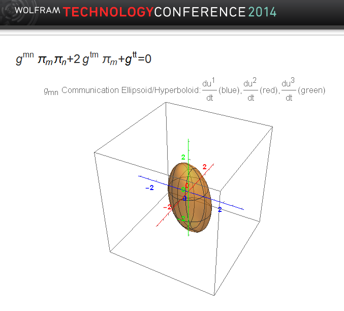
The idea that communication travels at a finite speed makes sense for any theory about our world, not just physics. But it has consequences when translated into differential geometry. There is a presumed measure of distance or metric between any two points given by the above rule. There is thus a relationship between the velocities or flows for maximal communication set by the surface in terms of this measure or metric:

What this means is that the maximum communication flow must lie on this ellipsoid. All communications must lie inside. This imposes constraints on the possible values of the metric elements, which must vary continuously from their initial values.
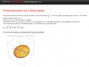
Here is a sample surface computed from the WWW model at a point. As one moves from point to point, the shape changes shape and can in fact turn into a hyperboloid. In Mathematica we use Manipulate to study this. A hyperboloid allows communications that occur at zero speed or infinite speed, neither of which are reasonable. Since the coefficients of the ellipsoid, the metric elements, are computed from the differential geometry equations, there are constraints on these metric elements.
We can gain additional insight by considering not just the velocity flow of communication, but the dual normalized  -flow:
It is the dual of the communication flow. We argued above that there was a difference between flow velocities related to the space and its dual. The dual was related to flows that we distinguished by whether the indices were upper or lower. Again, we are making that distinction here, to help us remember that this is not the flow but a linear combination of flow components. The requirement that communication be finite can be written in terms of these components and the inverse of the metric:


This shows the result for an initial point for the WWW model. Again, as we move away from this initial point, we require that the shape stay an ellipsoid. If we get zero or infinite flow, this is not physical. As before actual communication lies inside this ellipsoid. This imposes constraints on the inverse of the metric formed from the metric matrix elements  . Checking that we maintain the communication ellipsoid and its dual is easy and intuitive.
Summary
We have indicated several concepts that are distinct when we move to more complex geometries:
- Steady-state solutions can be more complex
- limit surfaces that are complex
- Chaotic behaviors
- Visualization challenges
- Dimensionality
- Gauge Invariance
- Conservation laws (symmetries)
- Normal versus orthogonal time
- Finite communication speed
- Communication ellipsoids
- Application to decision geometry
- WWW model
- Provides insight into decision-making
- Applications apply equally well to general relativity
- Speculation: can one extend these ideas to engineering?
- Especially the ideas of harmonics and harmonic series approximation

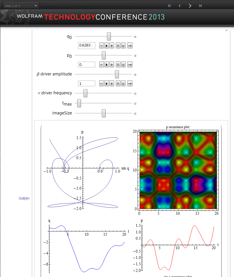
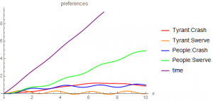 We have the following interpretation of this picture. From a game theory perspective, the model has two Nash equilibriums. The poor see their strategy to be “swerve” and assume that the wealthy will “crash”. The wealthy see the opposite. This is one variant of the classic game of chicken. It is clear in the figure that by assuming the wealthy are much less engaged, we are closer to one of the Nash equilibrium: we see the Nash equilibrium of the poor, which is to “swerve” and for the wealthy to “crash”.
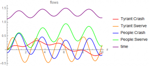
 that generalizes the vector potentials
  that determine the player payoffs, which are like the electric and magnetic fields in electrical engineering. In particular, if both points are active, then the tensor potential determines the frame transformation
  , whose differential is the flux flow through a 2-surface. The covariant and gauge invariant differential is
 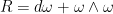 and the analogy is that this flow is zero through the surface.
 ; there is the purely inactive dimension flux flow
  ; and there is the purely active dimension flux flow
  . The constraints for each would be that the flow through the dual space
  is zero. This would imply for each case that
  with the appropriate changes in the subscripts.
 for the payoff fields on the boundary. A similar argument suggests imposing in addition the conditions
  for the inactive components and
  for the active components. As a consequence there will be some acceleration field flow through the surfaces. These are considered part of the initial “forcing functions” that may in fact yield insightful results about the decision process.
 .
.

 ; the eigenvalues are zero or purely imaginary.


 : this occurs when their distance scales
  is inactive. A related distinction is when the strategies
  form a coalition: this occurs when their sum is inactive. I think this can be generalized in a nice way to mean that these strategies form a surface. A special case is the constant sum game: the coalition consists of all players and their strategies. Although rather simple, I think these two distinctions revise both
 for any pair of “worldview” or inactive strategies
  , which is independent of these strategies. We have cooperative bonding when the strategies are different and value creation
  associated with
  when the strategies are the same. In our fixed frame model (
 . We have a geometric picture from the usual rules of calculus; the gradient is along the normal to the surface of constant potential. The tidal bond describes a potential field for each pair of players. Each player or code of conduct defines a symmetry transformation in the sense that none of the geometric constructs depend on the distance along the worldview (or code of conduct) direction. This extends to time as well if it too generates such a symmetry transformation.
 in a decision process is the sum over the value creation for each of the players. From the equations in decision process theory, the source for the total value creation is the energy density. Value creation reflects a tidal bond that is stronger the higher the energy density. Thus, we relate bonds (forces) to the exchange of value (energy). The potentials that are independent of the total value creation are the shear bonding potential
  where
where  in the theory is a diagonal matrix whose elements are all
  . The “trace” of the shear is zero, so in that sense it provides information that is distinct from the total value creation. It is interesting that in decision process theory, the shear bonding potential measures strain and is determined by the stress, generalizing physical theories where stress is proportional to strain.